Today, a look at Fresnel-modulated reflections. Hardly a secret trick, but it makes a surprising difference for somewhat shiny objects. Fresnel reflectance is the property that glancing reflections are stronger than head-on reflections. It’s particularly noticeable in surfaces like water or glass, but is even visible on a piece of paper. Oh, and since Fresnel reflectance is named after a person, it should always be capitalized (and since he was French, you don’t pronounce the ‘s’).
-
- Fixed blend factor between shading and environment
-

- Fixed blend factor between shading and environment
-

- Fresnel reflectance with a low dynamic-range environment texture
-

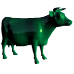
- Fresnel reflectance with a high dynamic-range environment texture
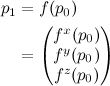
The most important directions for Fresnel reflectance are the surface normal, N, the direction you see the surface from, V, the direction the reflected light is coming from L (all unit-length vectors). Since it’s dealing with reflected rays, N should be half way between V and L, so N = normalize(V+L) and dot(N,V) = dot(N,L). I’m ultimately going to be applying it to an environment map, so I’ll stick with the dot(N,V) version.
There are also constants that control the strength of the effect: n1 and n2, the indices of refraction of each material, or sometimes rewritten in terms of n, the ratio of the two indices of refraction. Indices of refraction for common materials are pretty easy to find in a Physics text or online: vacuum is 1, air is pretty close to 1, water is about 1.33, glass is about 1.5.
Fresnel reflectance has different terms for incoming light polarized parallel to the surface than for light that’s not parallel to the surface. I’ll add another direction T, for the refracted light, since it makes the equations easier, though you can always rewrite the refracted direction in terms of the reflected one.
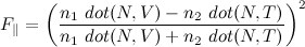
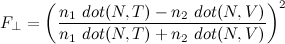
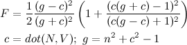
The polarization dependence is handy if you’re using a polarizing filter to enhance or diminish the reflections in a photograph, but most graphics assumes unpolarized light, which is an equal mix of both terms. Cook and Torrance came up with the combined form that was used in graphics for many years:
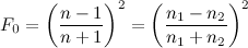
If you don’t have the index of refraction, it’s easier to measure the reflectance at normal incidence (looking head-on where it is smallest). From Cook and Torrance’s paper, that’s
But… almost everyone these days uses Schlick’s approximation for Fresnel. There’s actually lots of good stuff on approximating functions in Schlick’s paper, but only the Fresnel approximation seems to have really stuck:

For a little more intuitive control, you can write this in terms of F0 at normal incidence and F90 at the edge of the object:

Image d above is what it looks like for a high dynamic range environment map. I’ve also included a regular Blinn-Phong layer with a light source positioned at the brightest point in the environment texture. F is just the blend factor between the two.
It’s important to use a high-dynamic range texture for this, because ordinary 8-bit textures can’t distinguish between “the sky is bright”, maxed out at 255 and “the sun is 10,000 times brighter”, also maxed out at 255. Multiply by 0.04, and you get about 10 in both cases. But image was exposed so the sky really is 255, the sun should be around 25,500,000. When multiplied by 0.04, that’s still 10,200,000 (or really bright). If we don’t keep the full dynamic range of the environment map, we get the somewhat disappointing result in image c
Oh, and images a and b are what you get for a couple of choices of constant blend fraction. The glancing reflections around the edges of the model really add an extra dimension of shininess.