Short one today, just a note on nonlinear transformations. The usual translations, rotations and scaling transformations can all be described as a linear transformation (= matrix multiply). Even linear blend skinning, which blends between per-bone linear transformations is effectively piecewise linear. That basically means that each of x,y,z and w after transformation depend only on linear terms of x,y,z and w before transformation:
p1.x = a p0.x + b p0.y + c p0.z + d p0.w
Anything that includes higher powers of x,y,z or w, or some non-linear function is a nonlinear transformation:
p1.x = a2 p0.x p0.x + a1 p0.x + b p0.y/p0.w + c sin(p0.z)
I haven’t seen nonlinear transformations used too much in real-time graphics. There have been a few non-linear extensions to the linear blend skinning and some approaches for generating non-linear environment maps (e.g. paraboloid maps). They were popular for a time for free form deformation for production animation.
None the less, understanding what happens to points, tangents and normals helps explain where some of the well-known rules of graphics originate.
First, assume we’re transforming p0 to p1 by some function f:
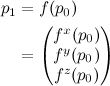
According to the rules of differential geometry, surface tangent vectors should transform by the Jacobian of the transform. The Jacobian is a matrix of partial derivatives (which I’ll indicate by subscripts, making my choice to label the components with superscripts above make a little more sense)
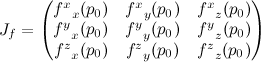
It depends on where p is, but it’s still just a matrix, so this is just a matrix multiply. I like to write tangent vectors as columns, so the multiply would look like this

Also, according to the rules of differential geometry, surface normal vectors should transform by the inverse Jacobian. I like to write normal vectors as rows, in which case the multiply would look like this:

One property of this is that the dot product of a normal and tangent are not affected by the transformation from one space to another (which is good):

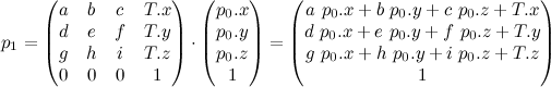
What does this have to do with ordinary linear transforms? Assuming no perspective, a linear transform looks something like this:
Dropping the constant row, the Jacobian of that guy is:
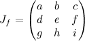
So that’s where “transform vectors by the upper left 3×3 corner of the transformation matrix” comes from. Similarly, we can understand transforming normals by the inverse transpose: inverse because it’s the inverse Jacobian, and transpose so you can multiply as a column on the right rather than a row on the left.
But… now we know how to do other nonlinear transforms, including what to do if this matrix actually has some perspective in it. Build a Jacobian matrix.
[Originally, this post attempted to use html for the math, which sucked. Updated to use LaTeX + MathURL]