Sometimes you want to uniformly distribute some objects over an area. Maybe they’re trees, maybe just blades of grass, maybe an army of guys. Whatever they are, there are a bunch of ways you could try. Here are a few.
-
- 256 points in a uniform grid
-
- 255 points on a hexagonal grid
-
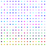
- 256 Hammersley points
-
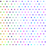
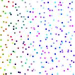
- 256 points with a uniform random distribution
-
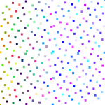
- 256 points with a jittered grid
-
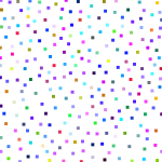
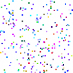
- 256 points in a Poisson disk distribution
These differ in the distribution of points and ease of generation. For distribution, the important characteristics are whether it’s clumpy or evenly spaced, as well whether it’s regular or more random. Ease of generation depends a lot on how you’re going to use it. If you can precompute positions, the complexity doesn’t matter too much. If computed at load time, the complexity might matter a little. However, sometimes you want to be able to quickly answer questions about the distribution without necessarily knowing the location of all the points. That could be “where is point n” (useful for shader-based instancing), or “are there any points near here” (useful for generating partial layouts, or proximity queries).
Easiest (and ugliest) is the uniform grid. If these were tree positions, they might do for an orchard, but would look really strange for a natural forest. You can easily find point n without placing all of the other points, and just as easily find nearby points by searching the neighboring grid cells.
We could do a little better on the layout with a hexagonal grid, since that’s the natural tightest packing on the plane. The points lie in little equilateral triangles. To keep the spacing even, we need to squish the vertical spacing by the height of an equilateral triangle, sqrt(3/4) ≈ .866. To keep about the same density, it comes out to s=sqrt(sqrt(3/4)) fewer rows in y and 1/s more columns in x. The closest integer layout near 16×16 is 15×17, so we have one fewer point. Since this is basically a skewed grid, it is still easy to find point n independently of the other points, and also not too hard to find nearby points. However, it’s still pretty regular, with all the points in nice neat rows.
The last of the deterministic layouts is a Hammersley sequence, one example of a quasi-random sequence. For Hammersley points, the x is just the point number, and y is the point number with the bits reversed. There are definitely still patterns, but no long rows of points. Once again, it is easy to find the location for point n, but much harder to find nearby points. They’ll be near in sequence to n, which guarantees their x is close, but some of those points will have vastly different y. You can play some bit tricks to reduce the search set, or just sweep through the points nearby in x.
The rest of the examples are all different flavors of random distributions. The first chooses each x and y as independent uniformly distributed random numbers (= calls to random() or rand() or drand48() or whatever your random number generator you happen to be using). Since the points are each independent, in theory point n shouldn’t depend on any of the other points. In practice, random number generators keep some state and return numbers in a sequence. That means for most random number generators, you’ll have to run through points 0 to n-1 before you can get the location of point n. There are stateless random number generators (see our High Performance Graphics paper for example), which let you break that artifical dependence and get the points in any order. Nearby points are hard to find without some auxillary data structure though, since any point in the list may be near point n. Also, the independence introduces some heavy clumping, which is usually not good.
The jittered one avoids some of the clumping by going back to the grid. Each point is placed in a random location within its grid cell, but every grid cell has a point and only one point appears in any grid cell. With a stateless random number generator, you can place point n without dependence on the other points. However, now proximity tests are once again possible by looking at the positions in nearby cells. Since the points may appear anywhere in their cell, you need to look at all cells that intersect the search radius. Jittered grids do have some clumping though, since “anywhere in the grid cell” could include four points all landing near the same corner.
The last example is a Poisson disk distribution. This is a random distribution where each point is no closer than a given radius to any other point. There are gobs of algorithms for generating these, though all that I know of require pre-generating the entire distribution. This particular plot was created with a dart-throwing algorithm, where you choose a random location, toss it out if it is too close to any previously placed points, then try again. Dart throwing is about the least efficient way to generate a Poisson distribution, but it’s easy to find other more efficient algorithms. You usually need to create some spatial data structure to help find nearby points, so if you keep that structure around, proximity queries are not too bad. Actually, jittered grids were first introduced to graphics as an approximation to the Poisson disk distribution, though the real thing is clearly much more evenly distributed.
If you’re curious, all of these were created with a point-placement vertex shader. Random numbers were two iterations of TEA (the Tiny Encryption Algorithm, see the above paper) on the point index. The blue component of the color is the point index, while red and green are randomly chosen based on the index.