Quaternions are an extremely handy representation for rotations. Unfortunately, they fall into a slightly dusty corner of math, so often seem just a little scary. It’s good to understand what they mean, at least for rotations, when it makes sense to them, and when it makes more sense to use rotation matrices. Euler angles occasionally make sense as an interface for specifying rotation, but please convert them to something else as soon as possible!
Quaternions are a combination of a 3D vector and a scalar. Rotation by an angle θ around a unit vector v is represented by the quaternion
q = vec4(sin(θ/2)*v, cos(θ/2))
The quaternion, q, will be unit length (the sum of the squares of all for components is one). You can easily look at a quaternion and tell the axis it rotates around by looking at the vector part, which won’t be unit length anymore since it is scaled by sin(θ/2), but still points in the right direction. You can tell the angle by either looking at the scalar part, or the length of the scaled vector part. The inverse rotation will have the axis pointing in the opposite direction, which you can think of as either a rotation around the opposite axis, or the result of flipping the sign of θ.
Interpolating rotations
One great thing about quaternions is how well they interpolate between two rotations. If you just linearly interpolate and re-normalize, you get a nice interpolation of rotation axes along a great circle, plus a smooth rotation of twists around those axes. For t in [0,1],
normalize( q1*(1-t) + q2*t )
In comparison, directly interpolating between rotation matrices gives you weird squishy non-rotations in the middle, and interpolating Euler angles tends to take you on odd paths, especially near the singularities.
You can do even better with the spherical linear interpolation or slerp, as straight linear interpolation goes faster in the middle than at the ends. There’s nothing quaternion-specific about slerp. Given two N-dimensional unit-length vectors, it’ll interpolate between them along an N-dimensional sphere. slerp between unit-length vectors q1 and q2 is given by
φ=acos(dot(q1,q2))
slerp(q1,q2,t) = q1*sin(φ*(1-t))/sin(φ) + q2*sin(φ*t)/sin(t)
That looks quite a bit like the linear interpolation, but with different mixing factors for q1 and q2. If the linear interpolate and renormalize isn’t good enough, but slerp’s trig functions are too slow, there are several approximations that land somewhere in between. My favorite is the one that does normal linear interpolation but replaces t with a polynomial to adjust the interpolation speed.
Using quaternions
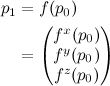
There are three main things to know for using quaternions. First, to rotate a single point p by quaternion q:
pRot = p + 2*cross(q.xyz, q.w*p + cross(q.xyz, p))
The second big operation is converting a quaternion rotation into a 3×3 rotation matrix. That’s
vec3 Q = 2.*q.xyz;
qMat = mat3(
 	1 - Q.y*q.y - Q.z*q.z, Q.x*q.y + Q.z*q.w, Q.x*q.z - Q.y*q.w,
 	Q.x*q.y - Q.z*q.w, 1 - Q.x*q.x - Q.z*q.z, Q.y*q.z + Q.x*q.w,
 	Q.x*q.z + Q.y*q.w, Q.y*q.z - Q.x*q.w, 1 - Q.x*q.x - Q.y*q.y);
The final big one is how to combine two quaternion rotations into a new one. That’s just
q = vec4(q1.w*q2.w - dot(q1.xyz,q2.xyz),
      q1.w*q2.xyz + q2.w*q2.zyx + cross(q1.xyz,q2.xyz));
So when do we use each? In raw operations, the direct quaternion rotation is 18 multiplies and 12 adds. GPU operations are at least somewhat dependent on the GPU, but assuming up to a four-element multiply-and-add or dot product is a single operation, it’s probably about 6 GPU instructions. That’s two for the inner cross product, one more to add in q.w*p, two more for the outer cross product, and one more to multiply by 2 and add to p.
The matrix construction, assuming the common multiplies are factored out, is 12 multiplies and 12 adds, while the matrix multiply to actually rotate with it would be 9 multiplies and 6 adds, for a total of 21 multiplies and 18 adds (clearly more expensive). In GPU terms, it’s about 7 GPU instructions to create the matrix and 3 to use it (still more expensive). On the other hand, to apply the same rotation to two points is 36 multiplies and 24 adds using the direct rotation, but only 30 multiples and 24 adds with the matrix multiply since you can use the same rotation matrix twice. So, to transform a single point, it’s best to use direct quaternion rotation, but for two or more (or even a point and normal), converting to a 3×3 matrix form is a big win.
Finally, combining two quaternions is 16 multiplies and 8 adds, or about 6 GPU operations. In comparison, combining two rotation matrices takes 27 multiplies and 18 adds or about 9 GPU instructions.
So… If you are doing lots of work with rotations, or need to do any interpolation between transformations at all, quaternions are the tool for you. If you are transforming more than one point by the resulting rotation, you’re better off converting the quaternion to a matrix to use it, but given that quaternions interpolate so much better and are so much cheaper to combine together, it’s still often worth it.
Perhaps in a later post I’ll go through the math behind quaternions, and how to get a quaternion given a rotation matrix, but for now, this is just enough quaternion to be dangerous.


\ \epsilon_B")


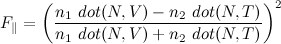
 won’t equal
  anymore, and it’s this difference that matters.
 - \left(\begin{matrix} B_x B_x & B_x B_y\\ B_x B_y & B_y B_y\end{matrix}\right)")
 , might come out negative due to numerical error (more on that later). If it is, I just clamp the matrix to 0. I like to add the specular power into the covariance at render-time, though you could add it into
  when creating the texture. Then the specular term is computed using a Beckmann distribution (basically a projected Gaussian distribution). Given Blinn-Phong specular power s, and normalized tangent-space light and view vectors Lt and Vt:
\\ Ht = \textrm{normalize}(Lt + Vt)\\ H = (Ht_x, Ht_y)/Ht_z - (B_x, B_y)\\ e = (H_x H_x Cov_{yy} - 2 H_x H_y Cov_{xy} + H_y H_y Cov_{xx})/\left|Cov\right|\\ spec = exp(-\frac{1}{2}e)/\sqrt{\left|Cov\right|}")

 and
and  are limited to -1 to 1, one bit in an 8-bit texture is 1/128, which limits the effective specular power to under 128. Compressed textures are out of the picture as the errors are just too big. So really, direct LEAN mapping is most useful if you have and can afford 16-bit textures.
(1-dot(H,V))^5")