UMBC Games, Animation and Interactive Media

Game Development at the University of Maryland, Baltimore County

Page 6 of 12

Graphics Trick: Quaternion Rotation

Quaternions are an extremely handy representation for rotations. Unfortunately, they fall into a slightly dusty corner of math, so often seem just a little scary. It’s good to understand what they mean, at least for rotations, when it makes sense to them, and when it makes more sense to use rotation matrices. Euler angles occasionally make sense as an interface for specifying rotation, but please convert them to something else as soon as possible!

Quaternions are a combination of a 3D vector and a scalar. Rotation by an angle θ around a unit vector v is represented by the quaternion

q = vec4(sin(θ/2)*v, cos(θ/2))

The quaternion, q, will be unit length (the sum of the squares of all for components is one). You can easily look at a quaternion and tell the axis it rotates around by looking at the vector part, which won’t be unit length anymore since it is scaled by sin(θ/2), but still points in the right direction. You can tell the angle by either looking at the scalar part, or the length of the scaled vector part. The inverse rotation will have the axis pointing in the opposite direction, which you can think of as either a rotation around the opposite axis, or the result of flipping the sign of θ.

Interpolating rotations

One great thing about quaternions is how well they interpolate between two rotations. If you just linearly interpolate and re-normalize, you get a nice interpolation of rotation axes along a great circle, plus a smooth rotation of twists around those axes. For t in [0,1],

normalize( q1*(1-t) + q2*t )

In comparison, directly interpolating between rotation matrices gives you weird squishy non-rotations in the middle, and interpolating Euler angles tends to take you on odd paths, especially near the singularities.

You can do even better with the spherical linear interpolation or slerp, as straight linear interpolation goes faster in the middle than at the ends. There’s nothing quaternion-specific about slerp. Given two N-dimensional unit-length vectors, it’ll interpolate between them along an N-dimensional sphere. slerp between unit-length vectors q1 and q2 is given by

φ=acos(dot(q1,q2))
slerp(q1,q2,t) = q1*sin(φ*(1-t))/sin(φ) + q2*sin(φ*t)/sin(t)

That looks quite a bit like the linear interpolation, but with different mixing factors for q1 and q2. If the linear interpolate and renormalize isn’t good enough, but slerp’s trig functions are too slow, there are several approximations that land somewhere in between. My favorite is the one that does normal linear interpolation but replaces t with a polynomial to adjust the interpolation speed.

Using quaternions

There are three main things to know for using quaternions. First, to rotate a single point p by quaternion q:

pRot = p + 2*cross(q.xyz, q.w*p + cross(q.xyz, p))

The second big operation is converting a quaternion rotation into a 3×3 rotation matrix. That’s

vec3 Q = 2.*q.xyz;
qMat = mat3(
 	1 - Q.y*q.y - Q.z*q.z, Q.x*q.y + Q.z*q.w, Q.x*q.z - Q.y*q.w,
 	Q.x*q.y - Q.z*q.w, 1 - Q.x*q.x - Q.z*q.z, Q.y*q.z + Q.x*q.w,
 	Q.x*q.z + Q.y*q.w, Q.y*q.z - Q.x*q.w, 1 - Q.x*q.x - Q.y*q.y);

The final big one is how to combine two quaternion rotations into a new one. That’s just

q = vec4(q1.w*q2.w - dot(q1.xyz,q2.xyz),
      q1.w*q2.xyz + q2.w*q2.zyx + cross(q1.xyz,q2.xyz));

So when do we use each? In raw operations, the direct quaternion rotation is 18 multiplies and 12 adds. GPU operations are at least somewhat dependent on the GPU, but assuming up to a four-element multiply-and-add or dot product is a single operation, it’s probably about 6 GPU instructions. That’s two for the inner cross product, one more to add in q.w*p, two more for the outer cross product, and one more to multiply by 2 and add to p.

The matrix construction, assuming the common multiplies are factored out, is 12 multiplies and 12 adds, while the matrix multiply to actually rotate with it would be 9 multiplies and 6 adds, for a total of 21 multiplies and 18 adds (clearly more expensive). In GPU terms, it’s about 7 GPU instructions to create the matrix and 3 to use it (still more expensive). On the other hand, to apply the same rotation to two points is 36 multiplies and 24 adds using the direct rotation, but only 30 multiples and 24 adds with the matrix multiply since you can use the same rotation matrix twice. So, to transform a single point, it’s best to use direct quaternion rotation, but for two or more (or even a point and normal), converting to a 3×3 matrix form is a big win.

Finally, combining two quaternions is 16 multiplies and 8 adds, or about 6 GPU operations. In comparison, combining two rotation matrices takes 27 multiplies and 18 adds or about 9 GPU instructions.

So… If you are doing lots of work with rotations, or need to do any interpolation between transformations at all, quaternions are the tool for you. If you are transforming more than one point by the resulting rotation, you’re better off converting the quaternion to a matrix to use it, but given that quaternions interpolate so much better and are so much cheaper to combine together, it’s still often worth it.

Perhaps in a later post I’ll go through the math behind quaternions, and how to get a quaternion given a rotation matrix, but for now, this is just enough quaternion to be dangerous.
Starry Eye is on the App Store

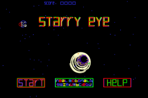
My game, Starry Eye, is on the App Store. It’s an arcade shooter, straight out of 1979. You play as the little blue guy with the tongue. Reviews wanted badly!

I’ve posted the entire project online at www.workly.com/starryeye/se10.zip

UMBC at Betascape.10

Thanks very much to Johnathan Moriarty, Eve Addison, Charles Lohr, Greg Aring, Fernando Lynch, Mary Lewis, Jenn Dahlke, and Bryan Eastlack for putting on a great show at the UMBC BetaScape table(s!) at ArtScape this weekend. I’m sure I forgot someone, please email me to let me know…

Brian Eastlack and Jenn Dahlke (both UMBC '10) demonstrating their game to Governor Martin O'Malley.

Brian Eastlack and Jenn Dahlke (both UMBC '10) demonstrating their game to Governor Martin O'Malley.

Congratulations to all on a show well-done!

Graphics Trick: Fresnel Environment

Today, a look at Fresnel-modulated reflections. Hardly a secret trick, but it makes a surprising difference for somewhat shiny objects. Fresnel reflectance is the property that glancing reflections are stronger than head-on reflections. It’s particularly noticeable in surfaces like water or glass, but is even visible on a piece of paper. Oh, and since Fresnel reflectance is named after a person, it should always be capitalized (and since he was French, you don’t pronounce the ‘s’).

The most important directions for Fresnel reflectance are the surface normal, N, the direction you see the surface from, V, the direction the reflected light is coming from L (all unit-length vectors). Since it’s dealing with reflected rays, N should be half way between V and L, so N = normalize(V+L) and dot(N,V) = dot(N,L). I’m ultimately going to be applying it to an environment map, so I’ll stick with the dot(N,V) version.

There are also constants that control the strength of the effect: n1 and n2, the indices of refraction of each material, or sometimes rewritten in terms of n, the ratio of the two indices of refraction. Indices of refraction for common materials are pretty easy to find in a Physics text or online: vacuum is 1, air is pretty close to 1, water is about 1.33, glass is about 1.5.

Fresnel reflectance has different terms for incoming light polarized parallel to the surface than for light that’s not parallel to the surface. I’ll add another direction T, for the refracted light, since it makes the equations easier, though you can always rewrite the refracted direction in terms of the reflected one.

F_\parallel=\left(\frac{n_1\ dot(N,V) - n_2\ dot(N,T)}{n_1\ dot(N,V) + n_2\ dot(N,T)}\right)^2
F_\bot=\left(\frac{n_1\ dot(N,T) - n_2\ dot(N,V)}{n_1\ dot(N,T) + n_2\ dot(N,V)}\right)^2

The polarization dependence is handy if you’re using a polarizing filter to enhance or diminish the reflections in a photograph, but most graphics assumes unpolarized light, which is an equal mix of both terms. Cook and Torrance came up with the combined form that was used in graphics for many years:

\begin{align*} F&=\frac{1}{2}\frac{(g-c)^2}{(g+c)^2}\left(1+\frac{(c(g+c)-1)^2}{(c(g-c)+1)^2}\right)\\ c&=dot(N,V);\ g=n^2+c^2-1 \end{align*}

If you don’t have the index of refraction, it’s easier to measure the reflectance at normal incidence (looking head-on where it is smallest). From Cook and Torrance’s paper, that’s

F_0=\left(\frac{n-1}{n+1}\right)^2=\left(\frac{n_1 - n_2}{n_1 + n_2}\right)^2

But… almost everyone these days uses Schlick’s approximation for Fresnel. There’s actually lots of good stuff on approximating functions in Schlick’s paper, but only the Fresnel approximation seems to have really stuck:

F=F_0 + (1-F_0)(1-dot(N,V))^5

For a little more intuitive control, you can write this in terms of F0 at normal incidence and F90 at the edge of the object:

F=F_0 + F_{90}\ (1-dot(N,V))^5

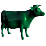
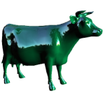
Image d above is what it looks like for a high dynamic range environment map. I’ve also included a regular Blinn-Phong layer with a light source positioned at the brightest point in the environment texture. F is just the blend factor between the two.

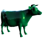
It’s important to use a high-dynamic range texture for this, because ordinary 8-bit textures can’t distinguish between “the sky is bright”, maxed out at 255 and “the sun is 10,000 times brighter”, also maxed out at 255. Multiply by 0.04, and you get about 10 in both cases. But image was exposed so the sky really is 255, the sun should be around 25,500,000. When multiplied by 0.04, that’s still 10,200,000 (or really bright). If we don’t keep the full dynamic range of the environment map, we get the somewhat disappointing result in image c

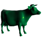
Oh, and images a and b are what you get for a couple of choices of constant blend fraction. The glancing reflections around the edges of the model really add an extra dimension of shininess.

Graphics Trick: GPU Random Numbers

This one is based on our recent High Performance Graphics Paper, “GPU Random Numbers via the Tiny Encryption Algorithm“, by Fahad Zafar, Aaron Curtis and Marc Olano.

Often you want a stream of random numbers in a shader. On the CPU, you usually have one stream of random numbers. Each time you ask, you get a new number. You might need to ask for new numbers a bunch for different things, but it doesn’t really matter if the requests for different purposes are all mixed up. On the GPU, you often want a bunch of independent streams corresponding to objects, characters, or grid cells in space. You want any GPU thread that asks for the random numbers associated with a particular stream to always get the same answers as a different thread asking for numbers from the same stream.

Several recent papers have used some kind of cryptographics hash for this. Cryptographic hashes are designed for things like signing messages, so the same input should always give the same result. That output should be pretty random (or someone might be able to crack the hash and sign fake messages, add viruses, or other nefarious things). We don’t care about the cryptographic security, but the other features are great for generating streams of random numbers: you put in the stream ID and a sequence number, and you get a random number. Since it’s a hash, every time you ask for the 5th number in the 1200th stream you get exactly the same answer.

The first graphics paper I know of to use this idea in graphics was my “Modified Noise for Evaluation on Graphics Hardware” from Graphics Hardware 2005. I used a modification of the Blum-Blum-Shub algorithm that pretty much destroyed all of its randomness, but made OK looking noise. In many ways, I was inspired by SGI’s lavarand, which encrypted an image of a bunch of lava lights to create random numbers (cool in its own right, though doesn’t really have the parallelization or repeatability). Tzeng and Wei (in “Parallel White Noise Generation on a GPU via Cryptographic Hash”, I3D 2008) used MD5, which was way more random than my stuff, but kind of slow. Our new paper uses the Tiny Encryption Algorithm (or TEA). TEA is actually a cipher rather than a hash, but for small input, it’s all the same. It repeats the same core mixing function for some number of rounds (64, when you’re using it for encryption). We show that lots of graphics tasks work well with just two rounds, but the more rounds you do the more random the results. After 8 rounds, it is random enough to pass both the DIEHARD and NIST randomness test suites.

For N rounds, it looks something like this:

uvec2 v = uvec2(stream, sequence);
uint s=0x9E3779B9u;
for(int i=0; i<N; ++i) {
    v.x += ((v.y<<4u)+0xA341316Cu)^(v.y+s)^((v.y>>5u)+0xC8013EA4u);
    v.y += ((v.x<<4u)+0xAD90777Du)^(v.x+s)^((v.x>>5u)+0x7E95761Eu);
    s += 0x9E3779B9u;
}
return v;

The s value is specified in the TEA algorithm, but the other hex constants are an encryption key, so could conceivably be changed to provide even more streams of random numbers.

For a streamlined two round version, I’d use something like this:

v.x += ((v.y<<4u)+0xA341316Cu)^(v.y+0x9E3779B9u)^((v.y>>5u)+0xC8013EA4u);
v.y += ((v.x<<4u)+0xAD90777Du)^(v.x+0x9E3779B9u)^((v.x>>5u)+0x7E95761Eu);
v.x += ((v.y<<4u)+0xA341316Cu)^(v.y+0x3C6EF372u)^((v.y>>5u)+0xC8013EA4u);
v.y += ((v.x<<4u)+0xAD90777Du)^(v.x+0x3C6EF372u)^((v.x>>5u)+0x7E95761Eu);

In fact, the pictures in my “distributing stuff” post were a bunch of points placed in a vertex shader using exactly that code. I happened to use OpenGL’s GLSL for that, but the Direct3D HLSL version looks almost identical, with uint2 replacing the uvec2.

Graphics Trick: Nonlinear transformations

Short one today, just a note on nonlinear transformations. The usual translations, rotations and scaling transformations can all be described as a linear transformation (= matrix multiply). Even linear blend skinning, which blends between per-bone linear transformations is effectively piecewise linear. That basically means that each of x,y,z and w after transformation depend only on linear terms of x,y,z and w before transformation:

p1.x = a p0.x + b p0.y + c p0.z + d p0.w

Anything that includes higher powers of x,y,z or w, or some non-linear function is a nonlinear transformation:

p1.x = ap0.x p0.x + ap0.x + b p0.y/p0.w + c sin(p0.z)

I haven’t seen nonlinear transformations used too much in real-time graphics. There have been a few non-linear extensions to the linear blend skinning and some approaches for generating non-linear environment maps (e.g. paraboloid maps). They were popular for a time for free form deformation for production animation.

None the less, understanding what happens to points, tangents and normals helps explain where some of the well-known rules of graphics originate.

First, assume we’re transforming p0 to p1 by some function f:

\begin{align*}
p_1 & = f(p_0) \\
& = \begin{pmatrix}
f^x(p_0) \\
f^y(p_0)\\
f^z(p_0)
\end{pmatrix}
\end{align*}

According to the rules of differential geometry, surface tangent vectors should transform by the Jacobian of the transform. The Jacobian is a matrix of partial derivatives (which I’ll indicate by subscripts, making my choice to label the components with superscripts above make a little more sense)

J_f=\begin{pmatrix}
{f^x}_x(p_0) _y(p_0) _z(p_0) \\
{f^y}_x(p_0) _y(p_0) _z(p_0) \\
{f^z}_x(p_0) _y(p_0) _z(p_0) \\
\end{pmatrix}

It depends on where p is, but it’s still just a matrix, so this is just a matrix multiply. I like to write tangent vectors as columns, so the multiply would look like this

t_1 = J_f \cdot t_0

Also, according to the rules of differential geometry, surface normal vectors should transform by the inverse Jacobian. I like to write normal vectors as rows, in which case the multiply would look like this:

n_1 = n_0 \cdot J_f^{-1}

One property of this is that the dot product of a normal and tangent are not affected by the transformation from one space to another (which is good):

dot(n_1,t_1) = n_1 \cdot t_1 = n_0 \cdot J_f^{-1} \cdot J_f \cdot t_0 = n_0 \cdot t_0 = dot(n_0,t_0)

What does this have to do with ordinary linear transforms? Assuming no perspective, a linear transform looks something like this:

p_1 = \begin{pmatrix}
a & b & c & T.x \\
d & e & f & T.y \\
g & h & i & T.z \\
0 & 0 & 0 & 1
\end{pmatrix} \cdot \begin{pmatrix}
p_0.x \\
p_0.y \\
p_0.z \\
1
\end{pmatrix} = \begin{pmatrix}
a\ p_0.x + b\ p_0.y + c\ p_0.z + T.x\\
d\ p_0.x + e\ p_0.y + f\ p_0.z + T.y\\
g\ p_0.x + h\ p_0.y + i\ p_0.z + T.z\\
1
\end{pmatrix}

Dropping the constant row, the Jacobian of that guy is:

J_f = \begin{pmatrix}
a & b & c \\
d & e & f \\
g & h & i \\
\end{pmatrix}

So that’s where “transform vectors by the upper left 3×3 corner of the transformation matrix” comes from. Similarly, we can understand transforming normals by the inverse transpose: inverse because it’s the inverse Jacobian, and transpose so you can multiply as a column on the right rather than a row on the left.

But… now we know how to do other nonlinear transforms, including what to do if this matrix actually has some perspective in it. Build a Jacobian matrix.

[Originally, this post attempted to use html for the math, which sucked. Updated to use LaTeX + MathURL]

Graphics Trick: Distributing stuff

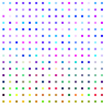
Sometimes you want to uniformly distribute some objects over an area. Maybe they’re trees, maybe just blades of grass, maybe an army of guys. Whatever they are, there are a bunch of ways you could try. Here are a few.

These differ in the distribution of points and ease of generation. For distribution, the important characteristics are whether it’s clumpy or evenly spaced, as well whether it’s regular or more random. Ease of generation depends a lot on how you’re going to use it. If you can precompute positions, the complexity doesn’t matter too much. If computed at load time, the complexity might matter a little. However, sometimes you want to be able to quickly answer questions about the distribution without necessarily knowing the location of all the points. That could be “where is point n” (useful for shader-based instancing), or “are there any points near here” (useful for generating partial layouts, or proximity queries).

Easiest (and ugliest) is the uniform grid. If these were tree positions, they might do for an orchard, but would look really strange for a natural forest. You can easily find point n without placing all of the other points, and just as easily find nearby points by searching the neighboring grid cells.

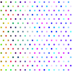
We could do a little better on the layout with a hexagonal grid, since that’s the natural tightest packing on the plane. The points lie in little equilateral triangles. To keep the spacing even, we need to squish the vertical spacing by the height of an equilateral triangle, sqrt(3/4) ≈ .866. To keep about the same density, it comes out to s=sqrt(sqrt(3/4)) fewer rows in y and 1/s more columns in x. The closest integer layout near 16×16 is 15×17, so we have one fewer point. Since this is basically a skewed grid, it is still easy to find point n independently of the other points, and also not too hard to find nearby points. However, it’s still pretty regular, with all the points in nice neat rows.

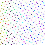
The last of the deterministic layouts is a Hammersley sequence, one example of a quasi-random sequence. For Hammersley points, the x is just the point number, and y is the point number with the bits reversed. There are definitely still patterns, but no long rows of points. Once again, it is easy to find the location for point n, but much harder to find nearby points. They’ll be near in sequence to n, which guarantees their x is close, but some of those points will have vastly different y. You can play some bit tricks to reduce the search set, or just sweep through the points nearby in x.

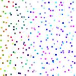
The rest of the examples are all different flavors of random distributions. The first chooses each x and y as independent uniformly distributed random numbers (= calls to random() or rand() or drand48() or whatever your random number generator you happen to be using). Since the points are each independent, in theory point n shouldn’t depend on any of the other points. In practice, random number generators keep some state and return numbers in a sequence. That means for most random number generators, you’ll have to run through points 0 to n-1 before you can get the location of point n. There are stateless random number generators (see our High Performance Graphics paper for example), which let you break that artifical dependence and get the points in any order. Nearby points are hard to find without some auxillary data structure though, since any point in the list may be near point n. Also, the independence introduces some heavy clumping, which is usually not good.

The jittered one avoids some of the clumping by going back to the grid. Each point is placed in a random location within its grid cell, but every grid cell has a point and only one point appears in any grid cell. With a stateless random number generator, you can place point n without dependence on the other points. However, now proximity tests are once again possible by looking at the positions in nearby cells. Since the points may appear anywhere in their cell, you need to look at all cells that intersect the search radius. Jittered grids do have some clumping though, since “anywhere in the grid cell” could include four points all landing near the same corner.

The last example is a Poisson disk distribution. This is a random distribution where each point is no closer than a given radius to any other point. There are gobs of algorithms for generating these, though all that I know of require pre-generating the entire distribution. This particular plot was created with a dart-throwing algorithm, where you choose a random location, toss it out if it is too close to any previously placed points, then try again. Dart throwing is about the least efficient way to generate a Poisson distribution, but it’s easy to find other more efficient algorithms. You usually need to create some spatial data structure to help find nearby points, so if you keep that structure around, proximity queries are not too bad. Actually, jittered grids were first introduced to graphics as an approximation to the Poisson disk distribution, though the real thing is clearly much more evenly distributed.

If you’re curious, all of these were created with a point-placement vertex shader. Random numbers were two iterations of TEA (the Tiny Encryption Algorithm, see the above paper) on the point index. The blue component of the color is the point index, while red and green are randomly chosen based on the index.

Akisakio is on the App Store!

Way to go, TeamSuperCool! Another UMBC student game, and they’ve got 60 reviews!

I’ve got it– of course. Akisakio is usually the first thing my kids run when I leave my phone within reach.

Graphics Trick: Homogeneous fun

Anyone who’s done any 3D graphics knows how to use homogeneous coordinates for translation and perspective, but they’re good for other places where you’d rather put off a division or avoid it entirely.

Basic homogeneous coordinates use four coordinates (I’ll use lower case to keep things straight) to represent a 3D point (here in upper case)

p = [x y z w]
P = [X  Y  Z] = [x/w  y/w  z/w]

Or more compactly, in shader notation

P = p.xyz / p.w

For regular points, we use w=1. If w=1/2, we get a point twice as far out in the p.xyz direction. If it’s 1/3, we get a point three times as far out in the p.xyz direction. In the limit, as w goes to 0, we get a point infinitely far away in the p.xyz direction.There’s no need to worry about a pesky division by 0, as long as we don’t ever actually have to do the division for the evil w’s.

That’s the basic idea behind my homogeneous rasterization paper (sometimes called clipless rasterization), used in quite a few GPUs. You normally compute the intersection between each triangle edge and a clipping plane to throw away the parts behind you where w might be 0 or negative. If you put off the division and keep everything in homogeneous coordinates long enough, eventually you can get all the way to visible pixels on the screen, with w’s guaranteed to be positive, before you actually have to divide.

But that’s not what this graphics trick is about. What else can we do using homogeneous coordinates to avoid division? Let’s say we want to subtract two points

V = Q – P = q.xyz/q.w – p.xyz/p.w

I can avoid dividing by putting that over a common denominator

V = (q.xyz * p.w  –  p.xyz * q.w) / (q.w*p.w)
v.xyz = q.xyz*p.w – p.xyz*q.w;  v.w = q.w*p.w

That lets either p or q be infinitely far away. So if P is a point on a surface, and Q is the location of a light, then V is a vector from the surface to the light (I’d use the traditional L, but lower-case l and number 1 tend to look a bit too similar). This will handle both point and directional lights with the same code. Of course, if you know a particular w is always 1 or always 0, you’d factor that constant into the equation in your code. Assuming p.w=1 to make things a little easier, for point lights (q.w=1), that reduces to a vector subtraction between the surface and light location

v.xyz = q.xyz – p.xyz;  v.w = 1

For directional lights, which are infinitely far away in a given direction (often used to approximate the sun), q.w=0, and we see the exact surface position doesn’t matter

v.xyz = q.xyz;  v.w=0

Also, though less common, you can use the same methods do parallel and perspective projection with the same code.

So that puts off the division and keeps everything in homogeneous coordinates, but in many lighting computations, you want a unit length vector pointing in the given direction

normalize(V) = V/length(V)

When you normalize, any scale factor that affects all three components has no effect on the final direction. If V is twice as long, or three times as long, or infinitely long, it still points the same way. In particular, as long as we avoid negative w’s, the division by v.w doesn’t affect the final direction, even if v.w=0.

normalize(v.xyz/v.w) = normalize(v.xyz) = normalize(q.xyz * p.w  –  p.xyz * q.w)

It’s amazing how far you can get with two simple rules: if the division might blow up, put it off. If a constant scaling won’t affect the result, don’t do it.

Marc

Graphics Trick: Polygon Area

This time, how about polygon area (plus circular loops).

The area of a 2D triangle is easy, it’s just half the magnitude of the cross product of two edges where you assume the z component is 0:

|cross((v1−v0),(v2−v0))|

The sign of the cross product tells you if the triangle is front or back facing (counter clockwise or clockwise). If you multiply out the cross product, it has an interesting repeating pattern if you collect it in terms with pairs of indices i and (i+1)%3

(v1.x−v0.x)*(v2.y−v0.y) − (v1.y−v0.y)*(v2.x−v0.x)
= v0.x*v1.y − v1.x*v0.y  +  v1.x*v2.y − v2.x*v1.y  +  v2.x*v0.y − v0.x*v2.y

As a bonus, for 3D triangles, the cross product points in the direction normal to the triangle, and its length is twice the area of the triangle. What’s more, the cyclical pattern appears again for each component (the order and signs here make more sense if you consider x,y,z to have their own mod cycle as well: x is followed by y is followed by z is followed by x …)

n.x = v0.y*v1.z − v1.y*v0.z  +  v1.y*v2.z − v2.y*v1.z  +  v2.y*v0.z − v0.y*v2.z
n.y = v0.z*v1.x − v1.z*v0.x  +  v1.z*v2.x − v2.z*v1.x  +  v2.z*v0.x − v0.z*v2.x
n.z = v0.x*v1.y − v1.x*v0.y  +  v1.x*v2.y − v2.x*v1.y  +  v2.x*v0.y − v0.x*v2.y

As a loop

n = float3(0,0,0);
for(int i0=0; i0<3; ++i0) {

int i1 = (i0+1)%3;

n.x += v[i0].y*v[i1].z − v[i1].y*v[i0].z;
n.y += v[i0].z*v[i1].x − v[i1].z*v[i0].x;
n.z += v[i0].x*v[i1].y − v[i1].x*v[i0].y;

}

Maybe overkill for a triangle, but the cool thing is that the same basic pattern works to find the area of any planar polygon with non-intersecting edges. It doesn’t even need to be convex. Just change the loop limit and mod from 3 to N. Just like the cross product, the magnitude will be twice the polygon area, and the sign will tell you if it is front or back facing.

Why does it work? It’s a simple application of Green’s theorum (or Stoke’s theorum in 3D). Bet you never thought you’d see that again, huh?

Mods add ugly unnecessary conditionals inside the loop, but if you shift the loop order a little, you can actually get rid of the mod:

for(int i0=N-1, i1=0;  i1<N;  i0=i1, ++i1) {

// loop order
// i0=N-1, i1=0
// i0=0,   i1=1
// i0=1,   i1=2
// …
// i0=N-2, i1=N-1

}

Extra bonus facts: in 3D, the resulting vector points in the direction of the polygon normal with length equal to twice the polygon area (just like the triangle cross product). Also, if you do it for the 1-ring of vertices around a given vertex (the vertices one edge away from a given vertex), you get exactly the triangle-area weighted average normal. Yes, that does mean that the area-weighted vertex normal doesn’t actually depend on the vertex position at all. Wierd, huh?

Marc

« Older posts Newer posts »